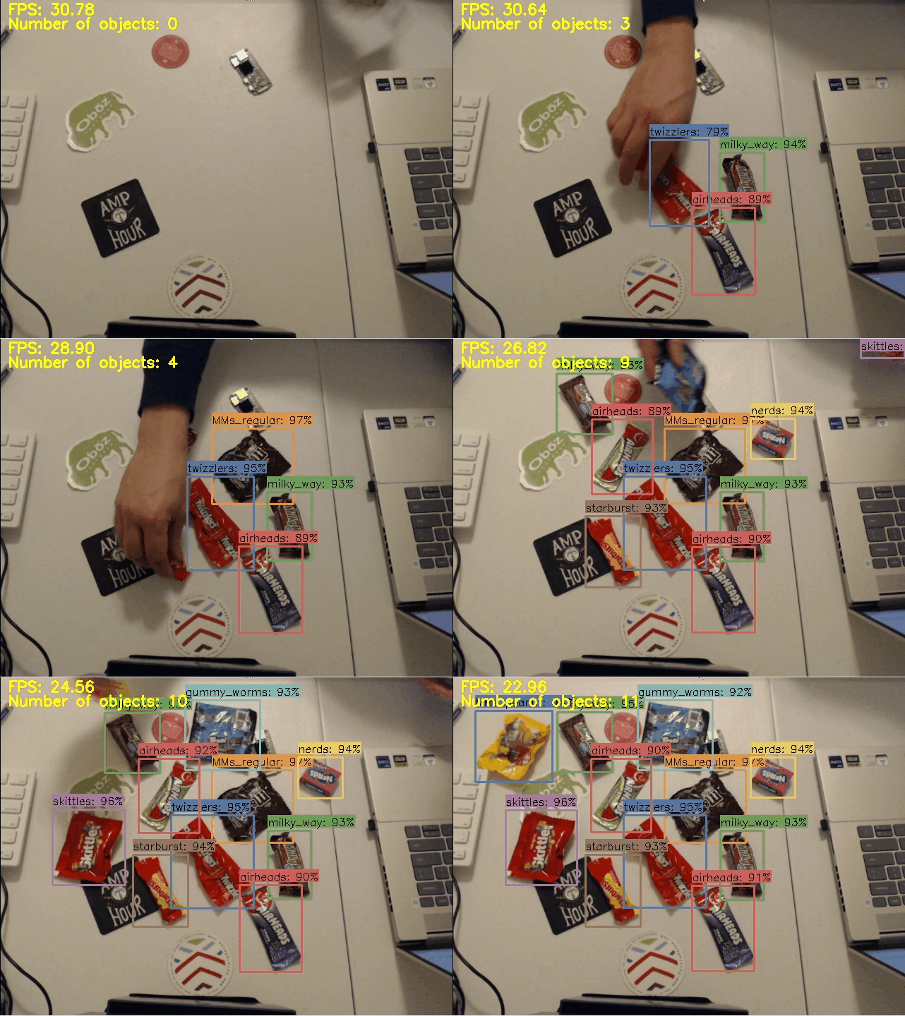
Ultralytics recently released YOLO11, a family of computer vision models that provides state-of-the-art performance in classification, object detection, and image segmentation. It utilizes an improved architecture that allows it to more accurately find object features and run faster than previous YOLO generations such as YOLOv8 and YOLOv5. Best of all, it is easy to train, convert, and deploy YOLO11 models in a variety of environments.

Figure 1. This article steps through the process of training a YOLO object detection model.
This guide provides step-by-step instructions for training (or fine-tuning) a custom YOLO11 object detection model on a local PC. It will go through the process of preparing data, installing Ultralytics, training a model, and running inference with a custom Python script. The guide shows how to run training on a local computer and graphics card (GPU). The guide is targeted for Windows PCs, but with some modifications, it can also be used for Linux or macOS systems. These instructions also work for training YOLOv8 and YOLOv5 models.
As an example, we’ll train a custom candy detection model that can locate and count the different types of candy in an image, video, or webcam feed. We’ll use images of popular candy (Skittles, Starburst, Snickers, etc.) to train the model.
NOTE: A CUDA-compatible NVIDIA graphics card is strongly recommended for training models. If you don’t have an NVIDA GPU, consider using our Google Colab notebook for training YOLO models instead, which allows you to run training on cloud-based GPUs. Most NVIDIA GeForce desktop and laptop cards will work for training models. A full list of CUDA-compatible graphics cards is available here.
Step 1 - Install Anaconda
First, we need to install Anaconda, which is a great tool for creating and managing Python environments. It allows you to install Python libraries without worrying about version conflicts with existing installations on your operating system.
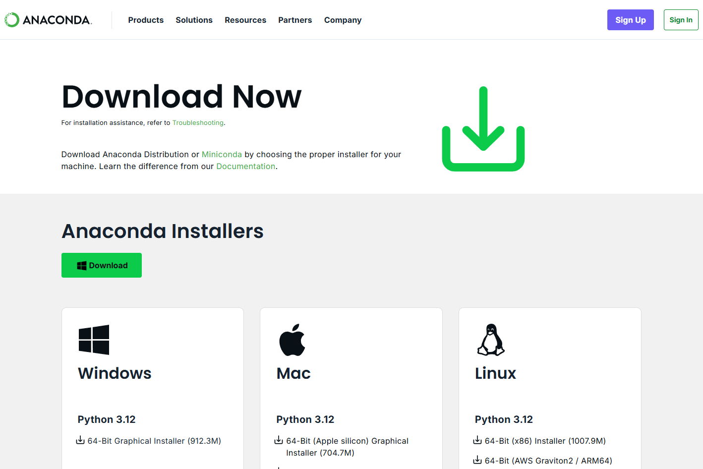
Figure 2. Download the Anaconda Installer for your OS from the Anaconda download page.
Go to the Anaconda download page at https://anaconda.com/download, click the “skip registration” button, and then download the package for your OS. When it’s finished downloading, run the installer and click through the installation steps. You can use the default options for installation.
Once it’s finished installing, search for “Anaconda Prompt” in the Start Bar and run it to open an Anaconda command terminal. We’ll work inside this terminal to install Python libraries and run training.
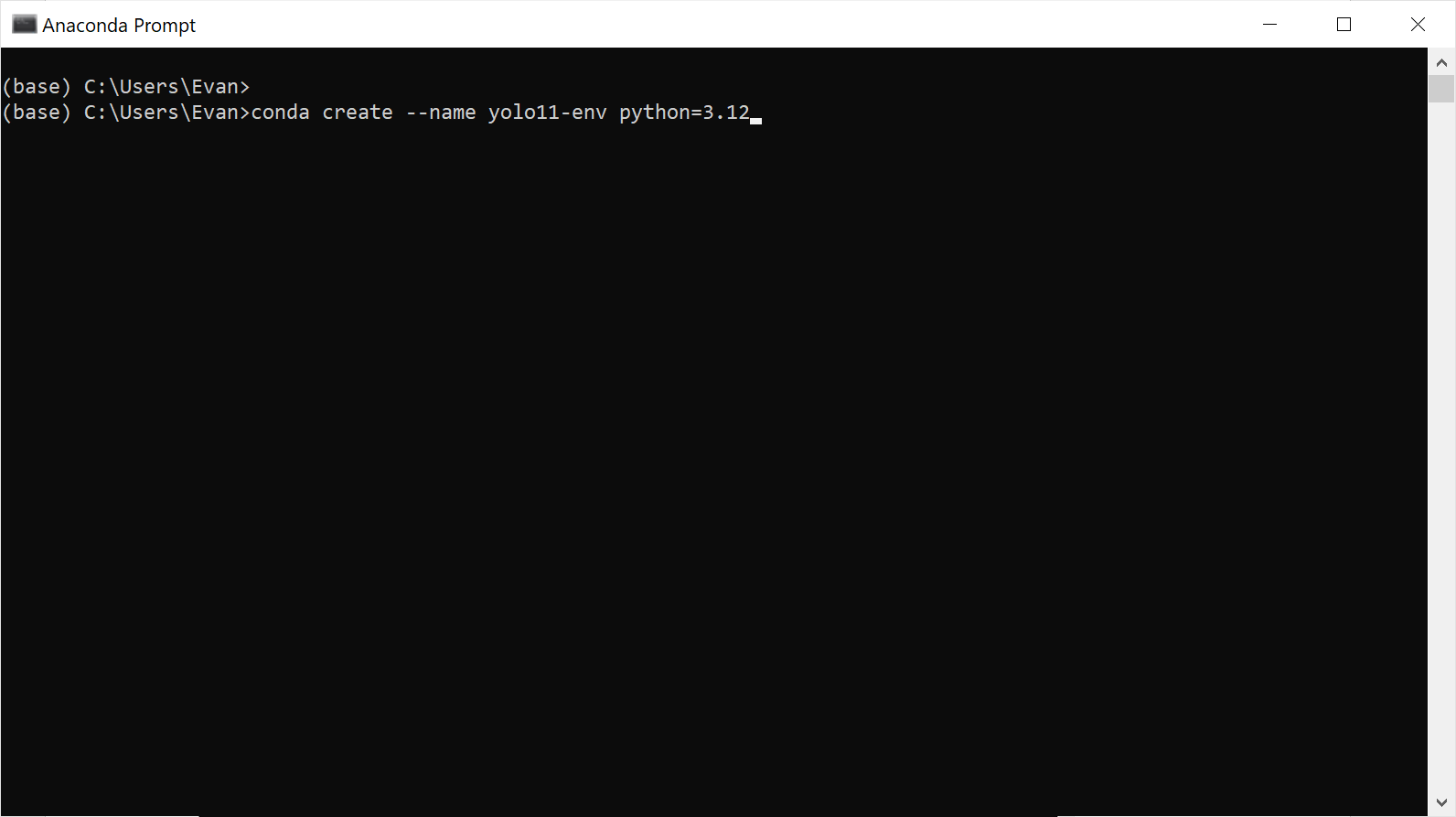
Figure 3. The Anaconda Prompt terminal we'll be working in throughout the guide.
Step 2 - Create New Environment and Install Ultralytics
Now, let’s create a new Anaconda Python environment for the Ultralytics library. Work through the following steps Create a new environment by issuing:
conda create --name yolo11-env python=3.12 -y
When it’s finished creating the environment, activate it by issuing:
conda activate yolo11-env
When it’s active, you’ll see the name of the environment in parentheses at the left of the command line. Next, we’ll install Ultralytics, a Python library for training and running YOLO models. Install it by issuing the following command. It downloads a large number of Python packages, so it will take a while.
pip install ultralytics
When installing Ultralytics, the Python package manager also installs several other powerful libraries, like OpenCV, Numpy, and PyTorch. It installs the CPU version of PyTorch by default. To run training on the GPU, we need to use the GPU-enabled version of PyTorch. Run the following command to install the GPU version of PyTorch:
pip install --upgrade torch torchvision torchaudio --index-url https://download.pytorch.org/whl/cu124
NOTE: PyTorch regularly releases updated versions with support for newer versions of CUDA. The command above installs PyTorch with CUDA v12.4. To see the command for installing the latest version, go to https://pytorch.org/get-started/locally/.
This command automatically installs the necessary versions of CUDA, cuDNN, and PyTorch-GPU inside the Anaconda virtual environment. It’s a very handy way to install CUDA drivers and libraries without having to go through the pain of downloading and installing them manually. You can confirm PyTorch-GPU is correctly installed by issuing the following command in the Anaconda Prompt terminal:
python -c "import torch; print(torch.cuda.get_device_name(0))"
If CUDA was installed correctly, this command will return the name of the GPU installed in your system.
Step 3 - Gather and Label Images
Before we start training, we need to gather and label images that will be used for training the object detection model. This guide will give a brief overview of the process, but for more detailed walkthrough on how to gather and label effective training images, see our article on the topic.
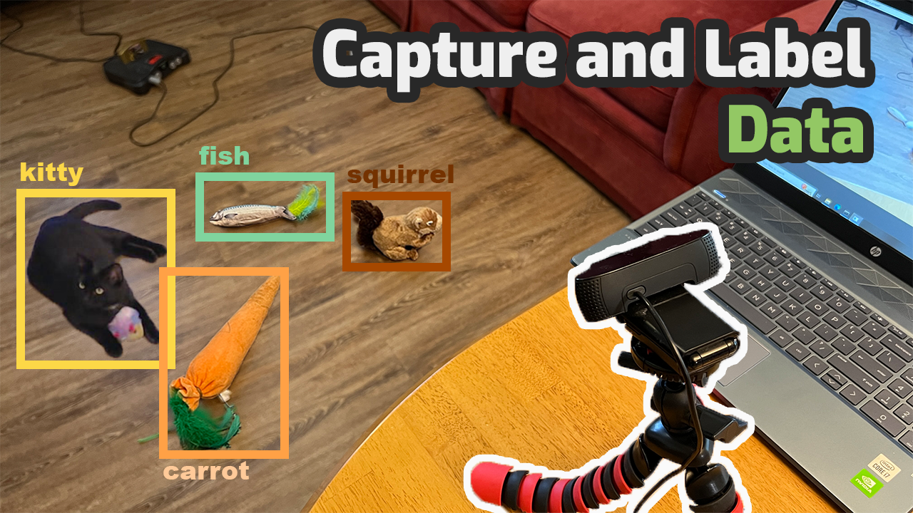
Figure 4. Click this image to visit our article that gives tips on how to gather and label images.
A good starting point for a proof-of-concept model is 100 to 200 images. The training images should show the objects in a variety of backgrounds, perspectives, and lighting conditions that are similar to what the model will see in the field. It’s also helpful to include other random objects along with the desired objects to help your model learn what NOT to detect.
NOTE: If you just want to try training a model, you can use our premade Coin Detection Dataset for the rest of this guide. It has 750 labeled images for training a model that will detect pennies, nickels, dimes, and quarters. Download it at this link and then continue to Step 4.
Once the images are gathered, label them using a labeling tool like LabelImg or Label Studio. Draw a box around each object in each image, making sure to fit the object tightly inside the label box. For more detailed instructions, see our YouTube video on training YOLO models, which shows how to label images using Label Studio.
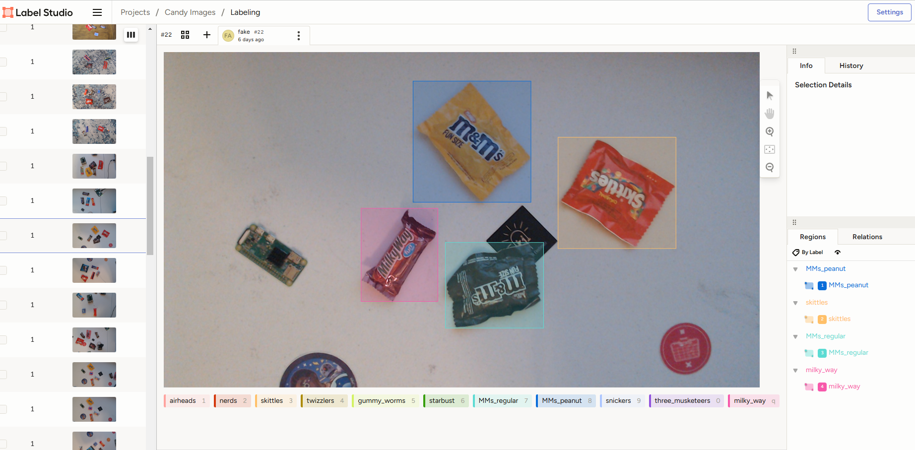
Figure 5. An example of a labeled image for the custom candy detection model
If you used Label Studio to label and export the images, they’ll be exported in a .zip file that contains the following:
- An “images” folder containing the images
- A “labels” folder containing the labels in YOLO annotation format
- A “classes.txt” labelmap file the contains the list of classes
Extract the .zip folder to a folder named “my_dataset” or similar. An example of the folder is shown below. If you obtained your dataset from another source (like Roboflow Universe or Kaggle) or used another tool to label your dataset, make sure the files are organized in the same folder structure (see my Coin Detection Dataset for an example).
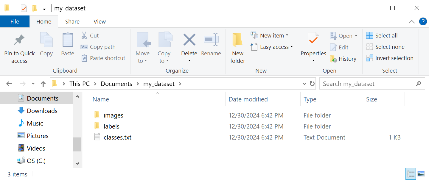
Figure 6. Organize your data in the folders shown here, where the images folder contains the training images, the labels folder contains annotation files, and the classes.txt file contains a list of classes.
In the next step, we’ll split these files into training and validation sets and organize them into the folder structure required for training YOLO models.
Step 4 - Set Up Folder Structure
Ultralytics requires a particular folder structure to store training data for models. The root folder is named “data”. Inside, there are two main folders:
- train: Contains the images and labels that are fed to the model during the training process. The training algorithm adjusts the model’s weights to fit to the data in these images.
- validation: Contains images and labels that are periodically used to test the model during training. At the end of each training epoch, the model is run on these images to determine metrics like precision, recall, and mAP.
Typically, 80% of the images in a dataset are split into the “train” folder, while 20% are split into the “validation” folder. In each of these folders is a “images” folder and a “labels” folder, which hold the image files and annotation files respectively.
The overall folder structure required for training Ultralytics YOLO models is shown below. In this section of the article, we’ll set up this folder structure using an automated Python script.
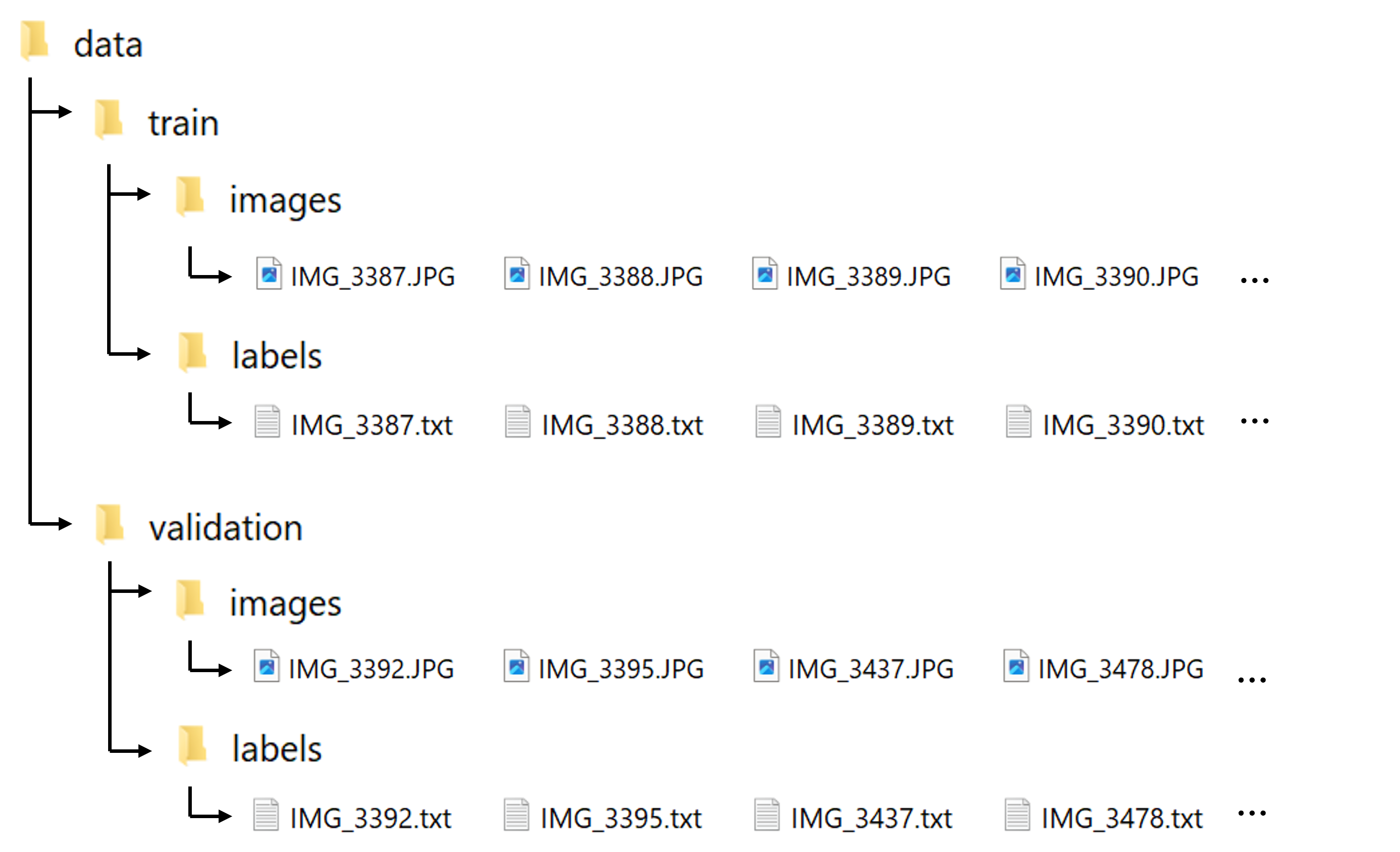
Figure 7. The Ultralytics library requires datasets to be in the folder structure shown here when training custom models.
4.1 Create root folder
We need to recreate the folder structure shown in Figure 7 before we train our model. Let’s start by making a folder to work from, where we’ll store both the data and the trained models. Create a folder named “yolo” in your Documents folder and move into it by issuing the following commands. Note, %USERPROFILE% points to your User folder in Windows (e.g., C:\Users\Evan):
mkdir %USERPROFILE%\Documents\yolo
cd %USERPROFILE%\Documents\yolo
Now you are working inside the C:\Users\username\Documents\yolo directory. We’ll use this directory as the working folder for the rest of the guide. Next, create the data folder by issuing:
mkdir data
You can manually move all the images and label files into the folder structure described above, or you can run our automated Python script to do it for you. The commands below show how to run the script, which will set up the folder structure and randomly split your images between training and validation.
4.2 Split dataset into train and val folders using automated Python script
First, download the script by issuing:
curl --output train_val_split.py https://raw.githubusercontent.com/EdjeElectronics/Train-and-Deploy-YOLO-Models/refs/heads/main/utils/train_val_split.py
Next, find the path to your folder from Step 3 containing the images and label files. For example, if the files are in a folder named “my_dataset” in your Documents folder, the path would be “C:\Users<username>\Documents\my_dataset”.
The “train_val_test.py” script has two arguments, “datapath” and “train_pct”:
- datapath : absolute path to the folder containing all the images and label files with double backslashes (example: “C:\\Users\\Evan\\Documents\\my_dataset”)
- train_pct : specifies the percentage for the train split (the remaining portion goes to validation). Typically, an 80%/20% train/val split is used (example:
.8)
Run the script by issuing the following command:
python yolo_train_val_split.py --datapath="C:\\path\\to\\data" --train_pct=.8
The script will go into the data folder, find every image (.jpg, .jpeg, .png, or .bmp) and label file (.txt), and randomly copy them into the train and validation folders. When the script finishes, your images and label files will be stored in the correct folder structure for training as shown in Figure 7.
Step 5 - Configure Training
There’s one last step before we can run training: we need to create the Ultralytics training configuration YAML file. This file specifies the location of your train and validation data, and it also defines the model’s classes. An example configuration file for my candy detection model is shown below.
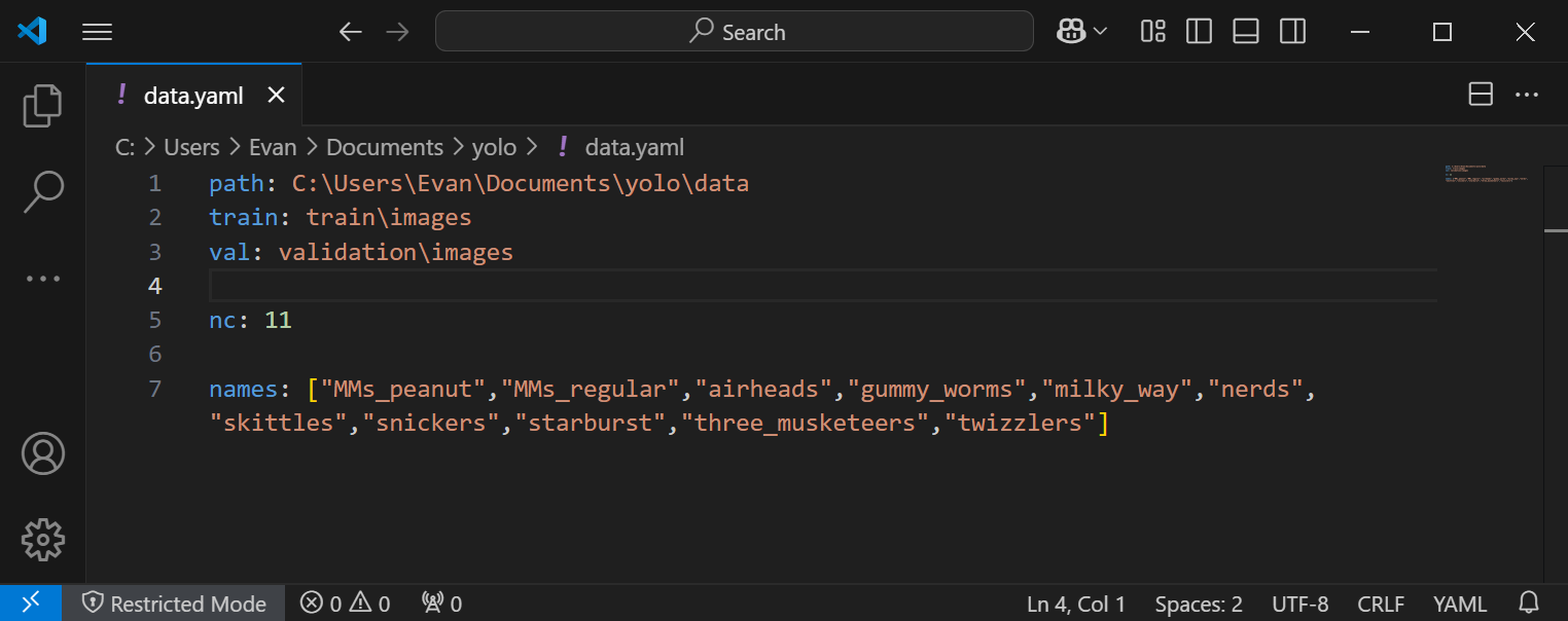
Figure 8. Example of the data.yaml configuration file for the candy detection model.
To create the configuration file, open a text editor such as Notepad and copy + paste the following text into it.
path: C:\Users\<username>\Documents\yolo\data
train: train\images
val: validation\images

nc: 5

names: ["class1", "class2", "class3", "class4", "class5"]
Make the following changes:
- Change “path:” to point at the data folder that was set up in Step 4 (e.g. C:\Users\Evan\Documents\yolo\data ).
- Change the number after “nc:” to the number of classes your model is being trained to detect (e.g. “4” if you are using the Coin Detection Dataset).
- Add the list of class names after “names:”. The classes should be in the same order of the labelmap defined in “classes.txt”. (e.g. [“penny”,”nickel”,”dime”,”quarter”] if you are using the Coin Detection Dataset).
Save the file as “data.yaml” in the “yolo” folder.
Once everything is configured, here’s what your “C:\Users\username\Documents\yolo” folder should look like.
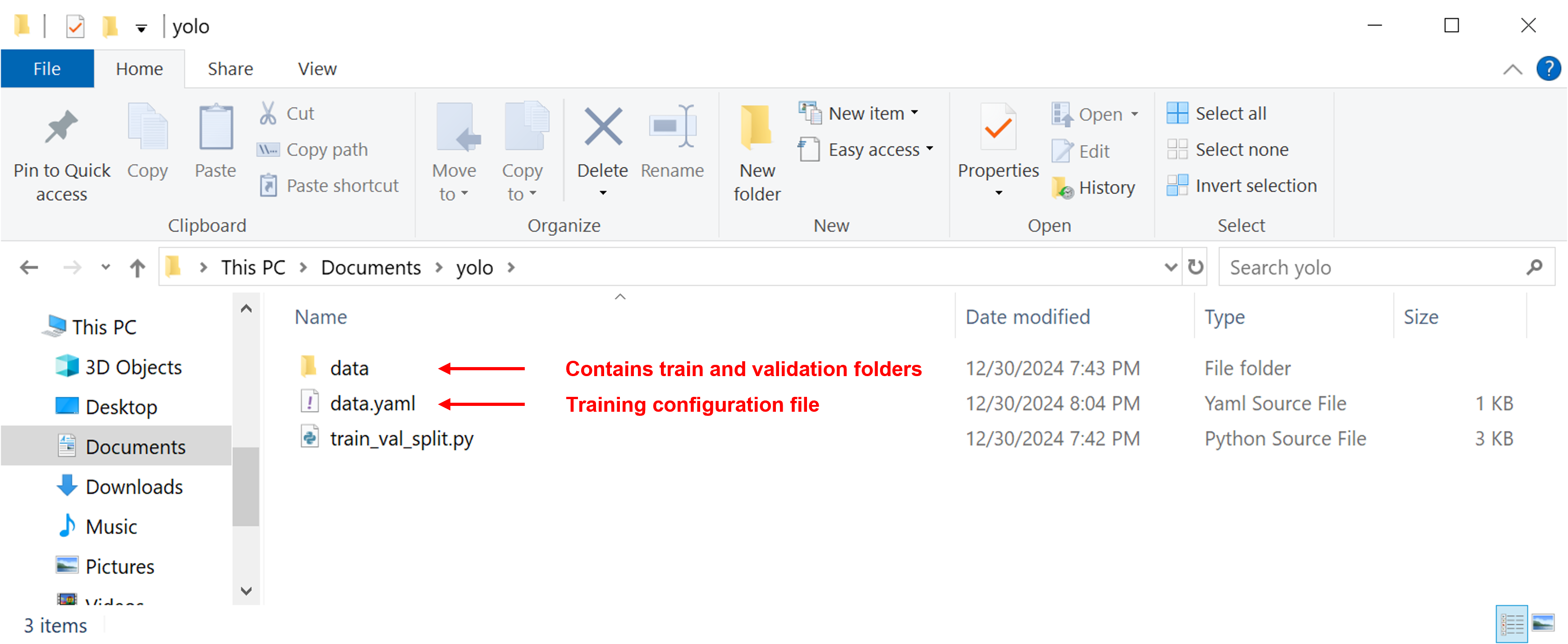
Figure 9. Contents of our working folder prior to training YOLO model.
Now that we have the data is in the correct folder structure and we created the training configuration file, we’re ready to start training!
Step 6 - Train Model!
Before we run training, there are a couple important parameters we need to decide on: which model to use and how many epochs to train for.
Selecting a model
There are a range of model sizes available to train. Information on the YOLO11 model options is listed in the table below (source: Ultralytics YOLO11 Performance Metrics).
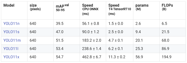
The important parameters to consider are mAP, params, and FLOPs. The mAP value indicates the relative accuracy of the model (i.e. how good it is at detecting objects) compared to the other models. The params and FLOPs columns indicate how “large” the model is: the higher these numbers are, the more compute resources the model will require. In general, the larger models run slower but have higher accuracy, while smaller models run faster but have lower accuracy. If you aren’t sure which model size to use, the “yolo11s.pt” model is a good starting point.
You can also easily train YOLOv8 or YOLOv5 models by just using “yolov8” or “yolov5” when running the training command. We did a comparison of different model sizes from the YOLOv5, YOLOv8, and YOLO11 families to test their relative accuracy and speed on two different datasets and hardware platforms. To see the results of our comparison, see our YOLO Model Performance Comparison video on YouTube.
Model resolution
YOLO models are typically trained and inferenced at a 640x640 resolution. The model’s input resolution can be adjusted using the “–imgsz” argument during training. Model resolution has a large impact on the speed and accuracy of the model: a lower resolution model will have higher speed but less accuracy. Generally, you should just stick with using the default 640x640 resolution. If you want your model to run faster or know you will be working with low-resolution images, try using a lower resolution like 480x480. Keep an eye on our Learn page for an article providing more information on training and inference resolution for Ultralytics YOLO models.
Number of epochs
In machine learning, one “epoch” is one single pass through the full training dataset. In each epoch, every image in the dataset is fed into the model, and the learning algorithm updates the model’s internal weights to better fit the data in the image. Typically, many epochs are needed for the model to adjust its weights to the data in the images.
Setting the number of epochs dictates how long the model will train for. The best amount of epochs to use depends on the size of the dataset, the model architecture, and the particular objects the model is being trained to detect. If your dataset has less than 200 images, a good starting point is 60 epochs. If your dataset has more than 200 images, a good starting point is 40 epochs.
For more information and tips on training models, see the Ultralytics Model Training Tips page.
Training the model
The “yolo detect train” command is used to run training. It has a few important arguments:
- data: specifies the path to the training configuration file (which we set up in Step 5)
- model: specifies which model architecture to train (e.g. “yolo11s.pt, “yolo11l.pt”). You can also train YOLOv5 and YOLOv8 models by replacing “yolo11” with “yolov5” or “yolov8” (e.g. “yolov5l.pt” or “yolov8s.pt”).
- epochs: sets the number of epochs to train for
- imgsz: sets the input dimension (i.e. resolution) of the YOLO model
Run the following command to begin training:
yolo detect train data=data.yaml model=yolo11s.pt epochs=60 imgsz=640
The training algorithm will parse the images in the training and validation directories and then start training the model. At the end of each training epoch, the program runs the model on the validation dataset and reports the resulting mAP, precision, and recall. As training continues, the mAP should generally increase with each epoch. Training will end once it goes through the number of epochs specified by “epochs”.
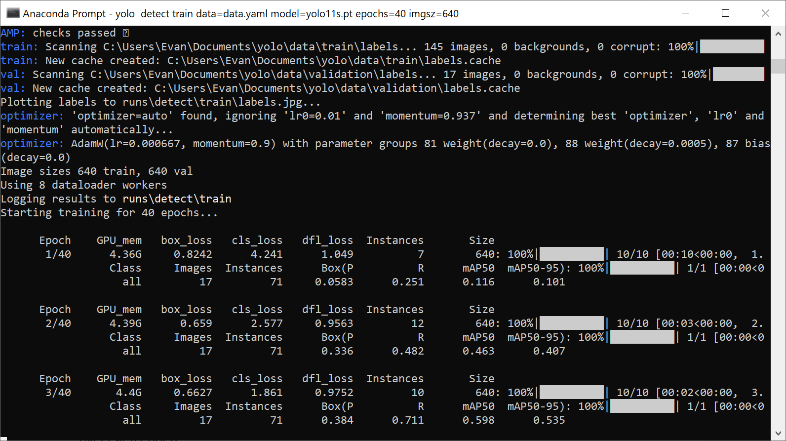
Figure 10. The progress of each training epoch will be reported as the training algorithm runs.
When training is finished (or if training is ended early with Ctrl+C), the trained model weights will be saved in “yolo\runs\detect\train\weights”. The “last.pt” file contains the model weights from the last training epoch. The “best.pt” contains the model weights from the training epoch that had the best mAP, precision, and recall. Generally, it’s recommended to use the “best.pt” model file for inference.
Additional information about training is saved in the “yolo\runs\detect\train” folder, including a “results.png” file that shows how loss, precision, recall, and mAP progressed over each epoch. If the mAP50 score doesn’t increase above 0.60, there is likely something wrong with your dataset (such as incorrect or conflicting labels).
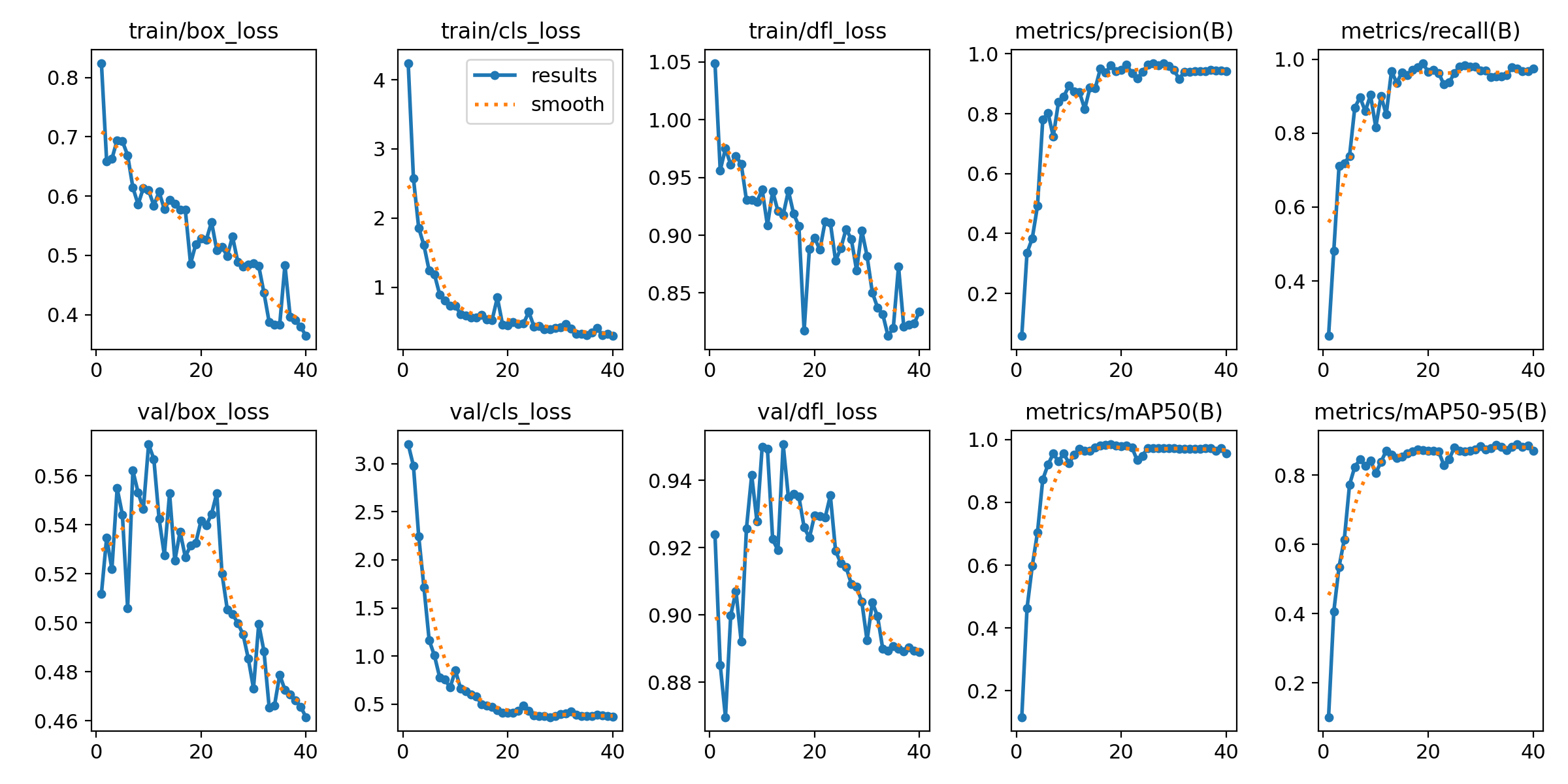
Figure 11. The results.png image shows how the model's loss, precision, recall, and accuracy progressed during training.
Step 7 - Run Model
Now that the model has been trained, let’s run it on some images, a video, or a live webcam feed!
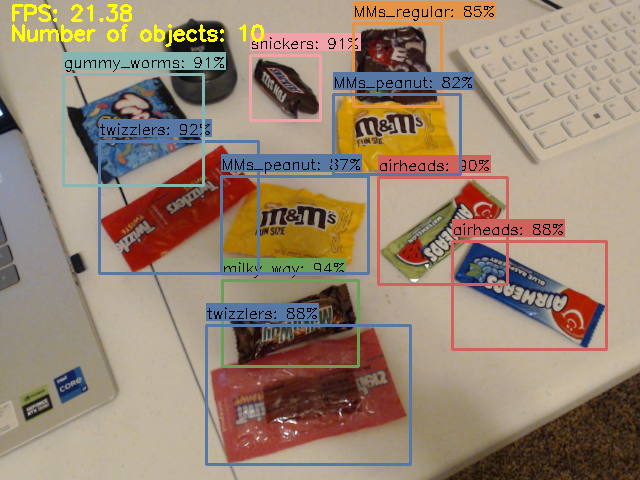
Figure 12. The candy detection model in action!
We wrote a basic Python script that shows how to load a model, run inference on an image source, parse the inference results, and display boxes around each detected class in the image. This script shows how to work with Ultralytics YOLO models in Python, and it can be used as a starting point for more advanced applications. Download the script to your PC by issuing:
curl -o yolo_detect.py https://raw.githubusercontent.com/EdjeElectronics/Train-and-Deploy-YOLO-Models/refs/heads/main/yolo_detect.py
The script takes two arguments, “model” and “source”:
- –model : Path to the trained model weights (e.g. “runs/detect/train/weights/best.pt”)
- –source: Path to a image file (“test_img.jpg”), a folder of images (“img_dir”), a video file (“test_vid.mp4”), or the index for a connected USB camera (“usb0”).
Here are example commands for running the script:
python yolo_detect.py --model=runs/detect/train/weights/best.pt --source=usb0  # Run on USB webacm
python yolo_detect.py --model=yolo11s.pt --source=test_vid.mp4 resolution=1280x720  # Run on test_vid.mp4 video file at 1280x720 resolution
When the script runs, it loads the model file and begin inferencing images from the image source. The script draws the detected bounding boxes on each image and displays it to the screen. Press “q” to stop the script.
Conclusions and Next Steps
Congratulations! You’ve successfully trained and deployed a YOLO object detection model. There are several things you can try next:
- Extend your application beyond just drawing boxes around detected objects. Add functionality like logging the number of objects detected over time or taking a picture when certain objects are detected. Check out some example applications at our GitHub repository: https://github.com/EdjeElectronics/Train-and-Deploy-YOLO-Models
- Deploy your model on the Raspberry Pi by following the instructions in our How to Run YOLO Detection Models on the Raspberry Pi article.
- Keep an eye on our Learn page and YouTube channel for articles and videos showing code examples and instructions for how to deploy YOLO models to other platforms.
If the model isn’t doing great at detecting objects, you can improve the model’s accuracy by adding more images to the training dataset. You should also review your training dataset to make sure there aren’t any mistakes with the labels.
EJ Technology Consultants has developed production-quality YOLO models for various applications, like traffic safety, casino game monitoring, hazard detection, and more. If you need help with any part of the model development process, whether it’s building a dataset, finding optimal training parameters, or deploying the model in an application, please contact us at info@ejtech.io or schedule a meeting on our Contact page. In the meantime, keep on training, and good luck with your projects!


